How Functional Ultrasound Works

Functional ultrasound · a primer from the Feng Lab

How functional ultrasound sees the brain working

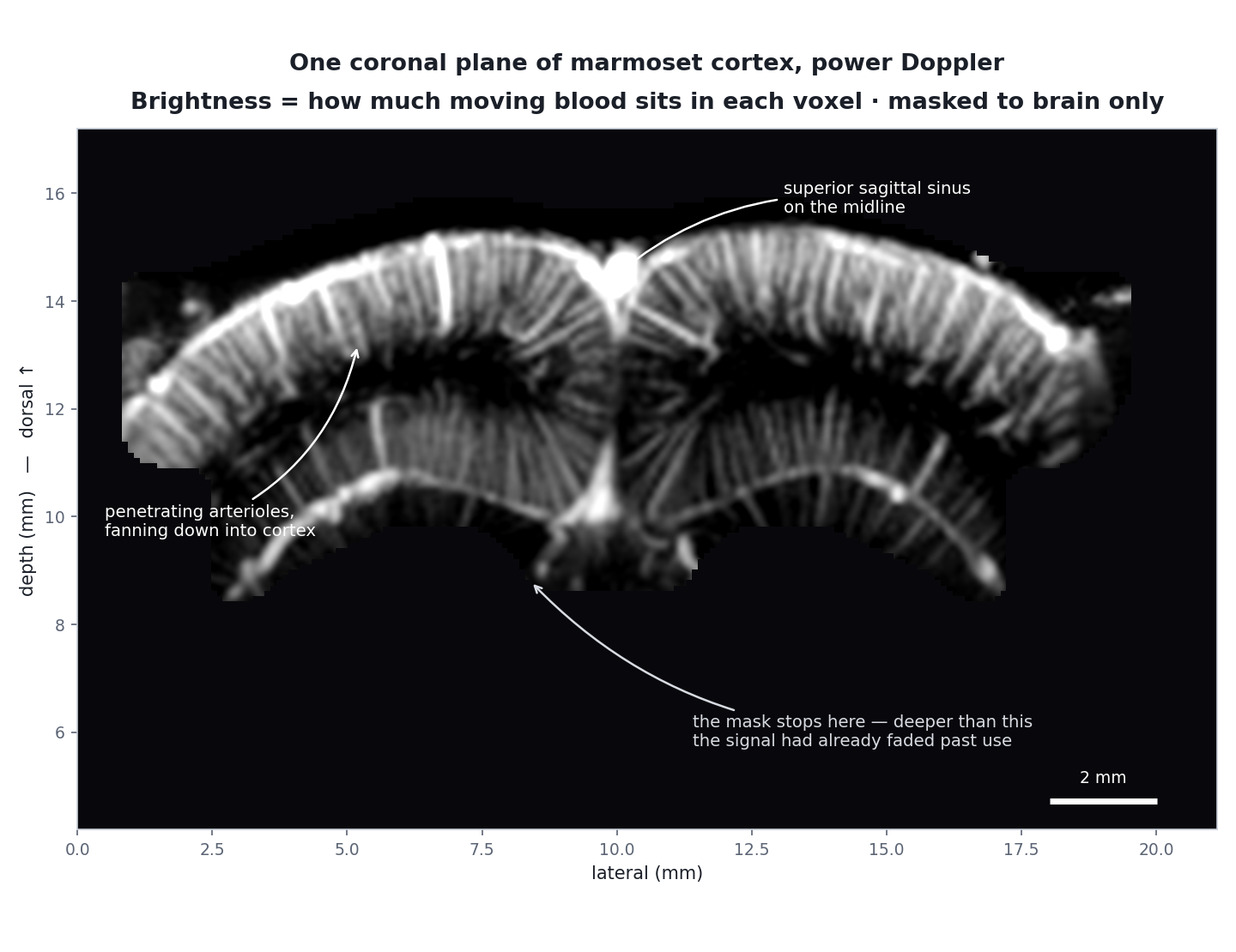
It doesn't image neurons. It images blood — fast enough, and sensitively enough, that the blood tells you where the neurons just fired. Here is the whole chain, from a sound pulse to a brain map, using real data from the volumetric fUS platform I'm building for behaving marmosets at MIT.

A coronal power-Doppler image of marmoset cortex, masked to the brain, showing the sagittal sinus at the midline and penetrating arterioles fanning down into cortex on both sides. — **This is a functional ultrasound image.** Not an anatomical scan with blood drawn on top — every bright thread is blood, and brightness is how much of it is moving in that voxel. It has been masked to the brain: ultrasound also images the scalp and muscle outside the skull, and those sit brightly at the edges of the raw frame with no relevance to anything here. What follows explains how a sound pulse becomes this picture, and then how the picture becomes a measurement of brain activity.

The premise

Why blood is a usable proxy for neural activity

When a patch of brain becomes more active, it needs more oxygen and glucose, and within a second or two the local vasculature dilates and delivers more blood to that patch. This is neurovascular coupling, and it is the same phenomenon fMRI relies on. Measure local blood volume over time and you have an indirect but reliable readout of where and when the brain is working.

Ultrasound is a good way to measure it. Sound passes through soft tissue, reflects off everything it meets, and — crucially — the echoes from moving red blood cells differ from frame to frame in a way that static tissue's echoes do not. The entire technique is built on separating those two things.

Step one

A pulse goes out, echoes come back, and timing gives you depth

The probe emits a very short burst of sound and then listens. Sound travels through tissue at about 1540 m/s, so an echo arriving later came from deeper down — 13 microseconds of round trip per centimetre of depth. One transmit gives you one line of brightness-versus-depth; an array of elements gives you a whole image plane.

That is all an ultrasound image fundamentally is: a map of how strongly each point in tissue reflected sound back at you.

Depth is inferred purely from arrival time. Nothing is focused mechanically and nothing moves — the probe stays still and the clock does the work.

Step two

Plane waves make it fast enough to be useful

Conventional ultrasound builds an image line by line: focus the beam on one line, listen, move to the next, repeat ~128 times. That costs 128 transmits per frame and caps you around 50 frames per second — far too slow to catch the subtle, fast fluctuations that blood flow produces.

Ultrafast imaging throws away the transmit focus. Fire a flat wavefront that floods the entire field at once, and a single transmit gives you a whole image — thousands of frames per second. The catch is that an unfocused transmit produces a poor image. The fix is coherent compounding: fire several tilted plane waves in quick succession and sum the reconstructed images, which synthesises a focus everywhere at once.

In the marmoset scans used here, that means 11 tilted plane waves spanning ±10°, summed into one frame, repeated 500 times a second.

The whole difference is what one transmit buys you. Tilting the flat wavefront and summing coherently recovers the image quality that dropping the transmit focus gave away.

Step three · the key distinction

B-mode looks at one frame. Doppler looks at how frames differ.

This is the distinction people most often get muddled, and it is simpler than it sounds.

B-mode — "brightness mode" — is the grey anatomical image everyone recognises from a clinical scan. Take the echo magnitude at every point in a single frame and display it. It shows structure: boundaries, membranes, tissue interfaces. What it does not show well is blood, because red blood cells are far weaker reflectors than tissue — roughly a thousand times weaker in returned power. In a B-mode image a blood vessel is typically a dark hole.

Doppler ignores any single frame and asks a different question: at this point in space, how did the echo change across a few hundred frames? Tissue sits still, so its echo repeats almost identically frame after frame. Blood moves, so its echo decorrelates rapidly. Collect 200 frames over 0.4 seconds and the two become separable — not by their strength, but by their behaviour over time.

The one-line version: B-mode measures how strongly a point reflects. Doppler measures how fast a point changes. Blood is invisible to the first and obvious to the second.

The clutter filter is the heart of the method. Tissue echoes are around a thousand times stronger than blood echoes, so they must be removed before blood is visible at all. Older systems used a simple high-pass filter in time, which also discarded the slowest — and most interesting — blood flow. Modern fUS instead decomposes the space-time matrix and drops the components that are spatially coherent, which is what tissue motion looks like. That change is most of why fUS can see small vessels.

B-mode versus Doppler, side by side

	B-mode	Doppler / fUS
Input	One frame	A few hundred frames in a row
Measures	Echo strength at each point	How fast the echo changes at each point
Shows	Tissue structure, boundaries, the skull	Moving blood, and nothing else
Blood appears as	A dark hole — red cells barely reflect	The entire signal
Time to form	Microseconds	0.4 s in these scans, set by the ensemble
Used here for	Placing the probe, checking coupling	Every measurement in the study

One real-world wrinkle worth knowing: the two modes need not even use the same transmit frequency. In one of the marmoset scans here, Doppler transmits at 12.5 MHz while B-mode transmits at 15.625 MHz — so quoting a single "probe frequency" for that scan would be wrong.

A note on the two Dopplers

Power Doppler, not velocity Doppler

"Doppler" covers two different outputs, and fUS almost always means the first:

Power Doppler takes the energy remaining after clutter filtering. It is proportional to how much moving blood sits in the voxel — roughly, blood volume. It carries no direction and no speed, it is relatively insensitive to the angle between the beam and the vessel, and it is what every image on this page shows.

Colour or velocity Doppler takes the mean frequency shift instead, giving speed and direction — flow towards or away from the probe. It is what clinical scanners overlay in red and blue. It is more angle-dependent and noisier, and in this project it appears only in a few dedicated velocity maps.

Step four

Repeat the measurement, and you have a functional signal

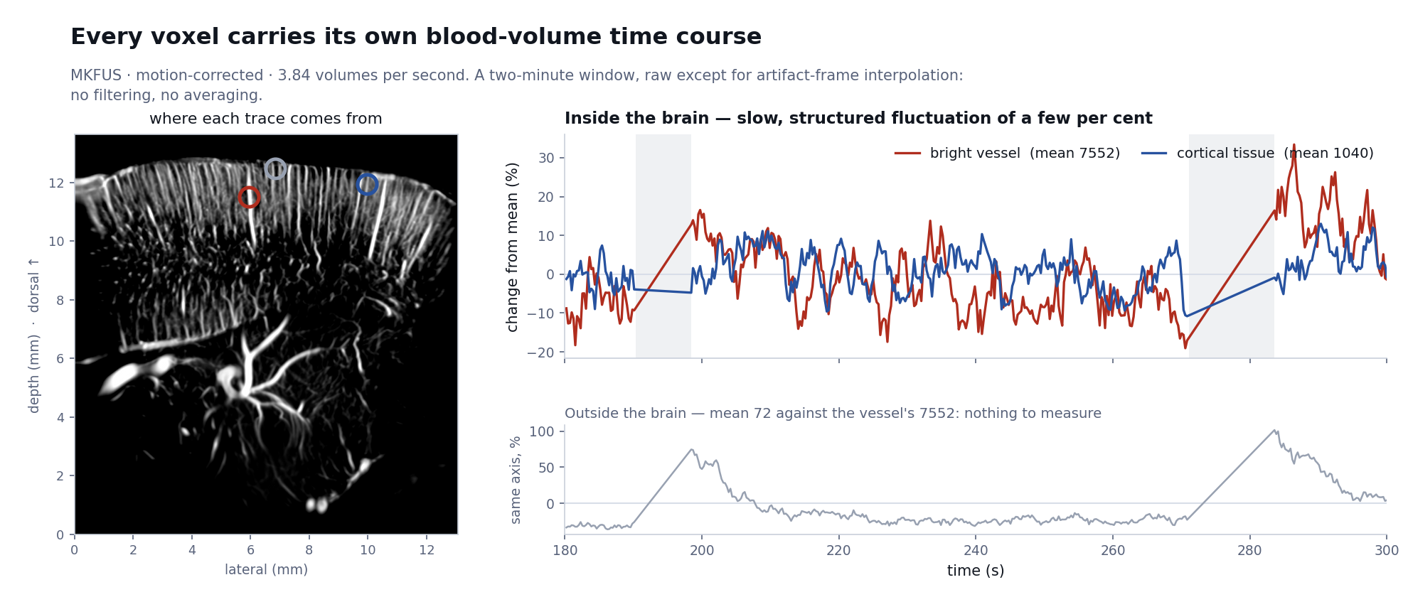
One power-Doppler image is an angiogram: a picture of the vasculature. Make one every few hundred milliseconds for minutes on end and each voxel acquires a time course — a running measure of how much blood is in that piece of brain, second by second. When the animal sees, hears or does something, the voxels serving the responsible region rise by a few percent within a second or two.

That is the functional measurement. It is the same logical step fMRI takes, with a different contrast mechanism: fUS measures blood volume directly rather than blood oxygenation, at finer spatial scale and with a faster response.

A coronal plane with three marked voxels and their power-Doppler time courses over a two-minute window: a vessel and a cortical voxel fluctuate by a few per cent with visible structure, while a voxel above the brain surface shows only low-level noise. — **Real traces, no filtering and no averaging.** The vessel and the cortical voxel fluctuate by a few per cent around their own means, and the fluctuation has visible structure rather than looking like noise — that is spontaneous haemodynamics. The third voxel sits just above the brain surface: its mean is 72 against the vessel's 7552, so there is simply nothing there to measure. Shaded bands mark stretches interpolated across motion-artifact frames. A stimulus-driven response would appear as a consistent rise in the first two traces, time-locked across repeats — which is exactly what the next section does.

A worked example

One real recording, from raw frames to an activation map

Everything above, applied end to end to a single session: one coronal plane of a marmoset receiving ten rewards over twelve minutes, sampled at 3.84 volumes per second. The file is 4.3 GB of power-Doppler frames. Every frame has been motion-corrected first, shifting it back into register — the animal moved by up to 23 pixels during the session, about 0.4 mm, which is the same order as the resolution itself.

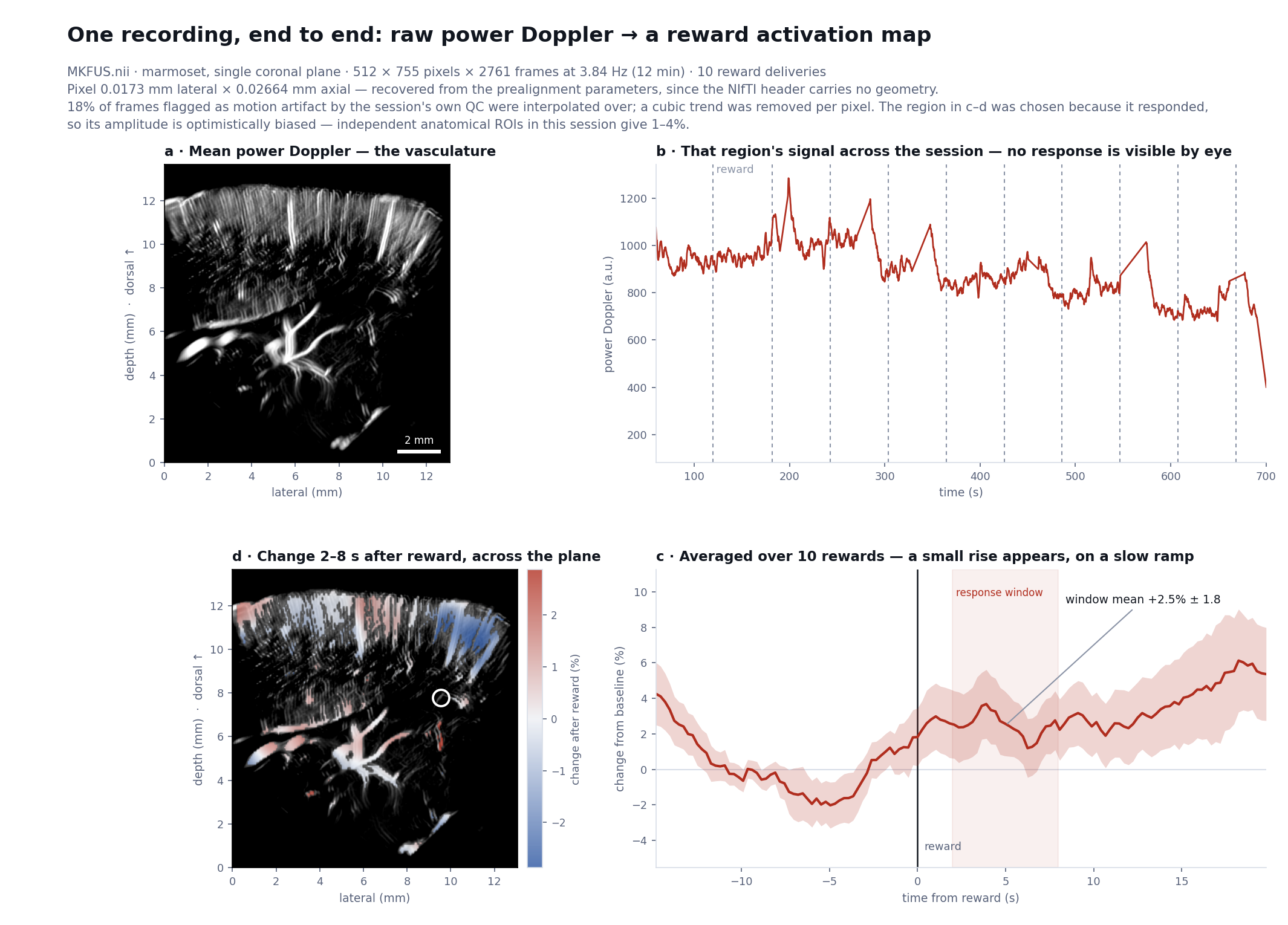
Four panels: the mean power-Doppler vasculature; one region's raw signal across the session with reward times marked; the trial-averaged response showing a small rise; and a map of change after reward across the plane. — **Panel b is the point.** The raw signal from the most responsive region, with every reward marked, shows nothing an eye can pick out. Only after averaging the same region across all ten rewards (panel c) does a rise appear at all — and it is **+2.5% ± 1.8**, which on its own is not statistically convincing. This is what real functional ultrasound data looks like before the polish.

Three things went wrong on the way to that figure, and all three are standard traps worth knowing before you trust anyone's activation map — including your own.

The trap	What it produced here	The fix
Motion left uncorrected	The animal shifted by up to 23 pixels across the session. Separately, 18% of frames were flagged bad by the session's own quality control — and every one of the brightest frames was among them. Left in, they swamped the real signal entirely.	Shift each frame back into register, then interpolate across the frames that are beyond saving — both before anything else.
Dividing by a near-zero baseline	A percent change needs a denominator. Computed on dim pixels, the first pass reported a 987% "response" — arithmetic, not physiology.	Require a real baseline signal, and normalise against a stable mean rather than a per-trial one.
Choosing the region by its own response	Take the maximum over thousands of noisy pixels and you have selected noise. Even after cleaning, the hand-picked spot reads higher than it should.	Define regions anatomically, independent of the data. Doing so in this session gives 1–4% — the honest number.

None of this is unique to ultrasound — it is the same circularity that fMRI spent years learning to control for. What is specific to fUS is how strong the artifacts are: the probe sits on a moving animal, and a brief movement can change the returned power by more than any brain response ever will.

Step five

Getting from a plane to a volume

A linear array images one plane. There are two ways to reach a volume, and this project has data from both.

The older approach translates the probe on a motor, imaging one plane at each stop. It gives excellent in-plane images over a wide field, but the planes are acquired at different times, so a "volume" is a mosaic rather than a snapshot — fine for anatomy, awkward for fast functional events.

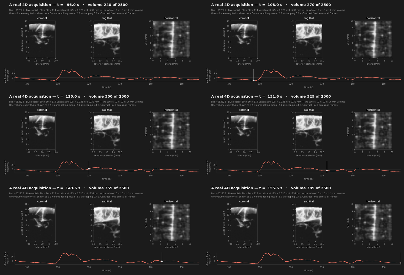
The newer approach uses a matrix array that steers electronically in both lateral directions, capturing a genuine volume every fraction of a second. The trade is field of view: the volumetric probe here covers 10 × 10 mm against the linear probe's 21 mm width.

The difference that matters for functional work is simultaneity: on the left, plane 51 is imaged well over a minute after plane 1.

An animation of a real four-dimensional functional ultrasound acquisition: coronal, sagittal and horizontal planes through the same 10 by 10 by 14 millimetre volume updating together across 150 volumes, with a cursor tracking position along the whole-volume mean signal below. — **What 4D actually looks like.** The same volume cut three ways, all updating together — because all three planes come from one electronically-steered acquisition rather than from separate passes. This is the whole 10 × 10 × 14 mm volume, nothing cropped, taken from a 16.7-minute session at one volume every 0.4 s. Contrast is fixed across every frame, so the brightness changes are real signal rather than autoscaling, and the slow swing in the trace below — tens of seconds long, tens of per cent deep — is haemodynamics, not noise. It is shown as a five-volume rolling mean stepping one volume, because a single volume on its own is sparse enough that only the brightest vessels survive, which is precisely why the functional measurement needs averaging.

A rotating maximum-intensity projection of the marmoset vasculature, showing surface vessels and the arterioles that descend from them into cortex, turning through a full revolution. — **The same data, turned around.** A maximum-intensity projection through the whole 10 × 10 × 14 mm volume, rotated a full revolution. This is what volumetric imaging buys you: the vessels running along the cortical surface, and the arterioles descending from them into the tissue, are one connected three-dimensional tree rather than a stack of unrelated pictures. Built from the mean of 300 volumes, so it shows the anatomy at the best signal-to-noise available — the *function* is the change in that anatomy over time, which the animation above shows. The bracketed corners mark the true bounds of the acquired volume and the coloured arrows the anatomical axes; both are computed from the same rotation that resamples the data, so they track it exactly. The volume does not fill its own box because signal fades with depth: that empty lower region is where the ultrasound stops reaching, not absent brain.

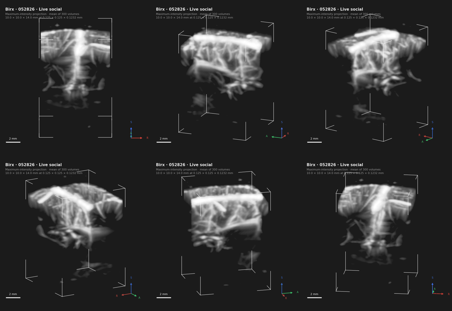
The numbers behind these images

Transmit12.5 MHz

Wavelength0.123 mm

Pulse2 cycles

Compounding11 × ±10°

Frame rate500 Hz

Ensemble200 frames

Per image0.4 s

Voxel0.11 mm

One caution for anyone about to write these down: voxel size is not resolution. The voxel is how finely the image is sampled, a choice made in reconstruction. Resolution is how close two vessels can be while remaining distinguishable, and it is set by wavelength, aperture and the compounding angles. They differ by several-fold, and the out-of-plane axis is always the worst of the three.

What it is good and bad at

The honest trade-offs

Higher frequency buys resolution and costs depth. Attenuation rises with frequency, so a 15 MHz probe resolves finer detail than a 12 MHz one but gives up penetration. In the images above, the signal fading below roughly 7 mm is attenuation — the anatomy is still there, the sound simply is not.

Bone is nearly opaque to ultrasound. This is the central practical constraint: fUS generally needs a thinned skull, a cranial window, or a species and age where the skull is thin enough to shoot through. It is why the technique took hold in rodents, neonates and intraoperative human work before adult non-human primates.

In exchange, you get something no other functional modality offers together: roughly 100 micrometre spatial scale, sub-second temporal resolution, direct blood-volume contrast, portable hardware, and compatibility with an awake, behaving animal.

References

Macé, E., Montaldo, G., Cohen, I., Baulac, M., Fink, M., & Tanter, M. (2011). Functional ultrasound imaging of the brain. Nature Methods, 8(8), 662–664. doi:10.1038/nmeth.1641
Montaldo, G., Tanter, M., Bercoff, J., Benech, N., & Fink, M. (2009). Coherent plane-wave compounding for very high frame rate ultrasonography and transient elastography. IEEE Transactions on Ultrasonics, Ferroelectrics, and Frequency Control, 56(3), 489–506. doi:10.1109/TUFFC.2009.1067
Demené, C., Deffieux, T., Pernot, M., et al. (2015). Spatiotemporal clutter filtering of ultrafast ultrasound data highly increases Doppler and fUltrasound sensitivity. IEEE Transactions on Medical Imaging, 34(11), 2271–2285. doi:10.1109/TMI.2015.2428634
Rabut, C., Correia, M., Finel, V., et al. (2019). 4D functional ultrasound imaging of whole-brain activity in rodents. Nature Methods, 16, 994–997. doi:10.1038/s41592-019-0572-y
Dizeux, A., Gesnik, M., Ahnine, H., et al. (2019). Functional ultrasound imaging of the brain reveals propagation of task-related brain activity in behaving primates. Nature Communications, 10, 1400. doi:10.1038/s41467-019-09349-w
Blaize, K., Arcizet, F., Gesnik, M., et al. (2020). Functional ultrasound imaging of deep visual cortex in awake nonhuman primates. PNAS, 117(25), 14453–14463. doi:10.1073/pnas.1916787117